- Published on
- 29 min read
The free wet-lab software stack: open-source replacements for GraphPad Prism, SnapGene, FlowJo, and BioRender
- Authors

- Name
- BioTech Bench
Table of contents
- The $6,000 software tax on a five-person bench
- What you'll learn
- 1. Replacing GraphPad Prism: R + ggplot2 + ggprism + SSfpl
- 2. Replacing SnapGene: OpenCloning + ApE + pLannotate + Biopython
- 3. Replacing FlowJo: FlowKit (Python) and flowCore / CytoExploreR (R)
- 4. Replacing BioRender: NIH BioArt + Bioicons + Inkscape + CellPAINT
- 5. Bonus: replacing paid image analysis and proprietary ELNs
- The master comparison table
- The real talk: where the free stack still loses
- My recommendation: how to actually migrate without a lab mutiny
- Resources
The $6,000 software tax on a five-person bench
Let me guess how software licensing works in your lab.
There is one computer near the gel doc with an active GraphPad Prism seat that three grad students take turns remoting into. Someone in the bay next to you is asking on Slack who currently has the plastic FlowJo USB dongle because the core facility's floating license server is full. Your plasmid maps live in a shared folder of .dna files that half the lab opens in the free SnapGene Viewer — until they actually need to simulate a Golden Gate assembly or design primers, at which point they borrow the postdoc's laptop. And two days before a manuscript goes out, someone realizes the figures they built on BioRender's free tier have watermarks and no publication license, so they pay $35 for a single month just to export the PDFs.
Sound familiar?
If you add up what a standard five-person academic wet lab actually pays for commercial desktop and cloud software — GraphPad Prism ($310–550/seat/year), SnapGene ($495–650/seat/year or a multi-seat lab pack), FlowJo ($550–1,200/seat/year), and BioRender ($420/seat/year for an individual academic plan) — you are looking at $5,000 to $8,000 every single year. For an industry startup paying commercial seat rates, multiply that by three or four.
Worse than the money is what happens when you leave. Walk out of a lab that runs on proprietary .pzfx, .dna, and .wsp files, and half your old analysis becomes read-only the day your institutional email expires.
Here is the honest answer about replacing that stack in 2026: you can replace 90% of it for $0, using free and open-source tools that produce better-documented, more reproducible science. But the last 10% comes with real friction, and anyone who tells you that switching from FlowJo or SnapGene to a script is completely painless is selling you something.
I went through the five biggest software categories in a molecular and cell biology lab, ran the open-source replacements on real bench workflows, and recorded the exact code and outputs below. Where the free tools beat the commercial incumbents, I'll show you how to set them up in ten minutes. Where they still fall short, I'll tell you plainly so you don't waste an afternoon.
What you'll learn
- How to get the exact GraphPad Prism look — plus four-parameter logistic (4PL) IC50 curves with profile-likelihood confidence intervals — in R with
ggprism,ggsignif, and basestats::SSfpl - Which free cloning tools actually replace SnapGene (
ApE,OpenCloning,pLannotate, andpydna+dna_features_viewer), with a runnable diagnostic digest and agarose gel simulation - How to gate
.fcsflow cytometry files and quantify CRISPR knock-in efficiency without FlowJo, usingFlowKitin Python orflowCore/CytoExploreRin R - How to build publication-licensed schematics and molecular figures without a BioRender subscription using
NIH BioArt,Bioicons,Inkscape,CellPAINT, andChimeraX - What to use for microscopy image analysis (
Fiji,CellProfiler,QuPath) and self-hosted lab notebooks (eLabFTW,BenchOS) - The honest trade-offs: where you should switch tomorrow, and where a paid seat is still worth keeping
1. Replacing GraphPad Prism: R + ggplot2 + ggprism + SSfpl
What you're paying now: ~$310–550/year per academic seat (more for commercial).
If you've read the R for Biologists learning path, you already know that t-tests and ANOVA in R take three lines of code, and that putting together a full qPCR workflow is faster in a script than clicking through eight Prism tabs.
When I ask bench biologists why they still keep their Prism subscription anyway, I almost always hear the same two answers:
- "My PI wants the graphs to look like Prism — thick black L-axes, outward tick marks, individual replicate dots on top of the bars, and significance brackets."
- "I need to fit sigmoidal dose-response curves and get an IC50 with 95% confidence intervals for my viability assays."
Both of those are solved problems in R, and neither requires a twenty-package dependency chain.
For the aesthetic, Charlotte Dawson's ggprism package wraps ggplot2 with theme_prism(), Prism color palettes, and offset minor-tick axis guides (guide_prism_offset_minor()). For the dose-response curves, base R's built-in stats package ships with SSfpl() — a self-starting four-parameter logistic model that fits the exact same four-parameter Hill equation Prism uses, with zero extra curve-fitting packages to install.
Let's run both side by side. First, install ggprism, ggsignif, and patchwork (if you don't have them alongside ggplot2, dplyr, and readr):
install.packages(c("ggprism", "ggsignif", "patchwork"))
Load the packages and pull in elisa_data.csv — a cytokine ELISA with three treatment groups (Control, Drug_1uM, Drug_10uM), three biological replicates per group, and two technical replicate wells per sample:
library(readr)
library(dplyr)
library(ggplot2)
library(ggprism)
library(ggsignif)
library(patchwork)

elisa <- read_csv("public/static/datasets/elisa_data.csv", show_col_types = FALSE)

# Average technical replicates first: 1 value per biological replicate (n = 3)
elisa_bio <- elisa |>
  group_by(group, biological_rep) |>
  summarise(od = mean(od_value), .groups = "drop") |>
  mutate(group = factor(group, levels = c("Control", "Drug_1uM", "Drug_10uM")))

print(elisa_bio)
# A tibble: 9 × 3
  group     biological_rep    od
  <fct>              <dbl> <dbl>
1 Control                1 0.201
2 Control                2 0.190
3 Control                3 0.208
4 Drug_10uM              1 0.897
5 Drug_10uM              2 0.882
6 Drug_10uM              3 0.905
7 Drug_1uM               1 0.486
8 Drug_1uM               2 0.500
9 Drug_1uM               3 0.481
Notice what we just avoided. In GraphPad Prism, it is dangerously easy to paste all six technical-replicate wells into a column table and run a one-way ANOVA as if . In R, grouping by biological_rep first forces you to treat technical duplicates as what they actually are: two measurements of the same biological sample.
Run the one-way ANOVA and Tukey HSD post-hoc test on those biological replicates:
fit_aov <- aov(od ~ group, data = elisa_bio)
print(TukeyHSD(fit_aov))
  Tukey multiple comparisons of means
    95% family-wise confidence level

Fit: aov(formula = od ~ group, data = elisa_bio)

$group
                        diff       lwr       upr p adj
Drug_1uM-Control   0.2896667 0.2633816 0.3159517 2e-07
Drug_10uM-Control  0.6946667 0.6683816 0.7209517 0e+00
Drug_10uM-Drug_1uM 0.4050000 0.3787149 0.4312851 0e+00
Now let's tackle the second reason people keep Prism: fitting a four-parameter logistic (4PL) dose-response curve to an 8-point inhibitor titration (1 nM to 10 µM, in biological triplicate) and extracting the and its profile-likelihood 95% confidence interval:
dose_df <- tibble(
  dose_uM = rep(c(0.001, 0.003, 0.01, 0.03, 0.1, 0.3, 1, 3, 10), each = 3),
  rep     = rep(1:3, times = 9),
  viability = c(
    99.4, 101.2, 97.8,
    98.1,  95.6, 99.0,
    92.3,  89.7, 94.1,
    78.4,  74.9, 80.2,
    51.2,  47.8, 53.5,
    24.6,  21.9, 27.1,
    11.8,   9.4, 13.2,
     7.2,   6.1,  8.4,
     6.5,   5.8,  7.0
  )
) |>
  mutate(log10_dose = log10(dose_uM))

fit_4pl <- nls(viability ~ SSfpl(log10_dose, Bottom, Top, logIC50, scal), data = dose_df)
coefs <- coef(fit_4pl)
ci_log <- suppressMessages(confint(fit_4pl, "logIC50"))

print(round(coefs, 3))
 Bottom     Top logIC50    scal
 99.732   5.490  -1.044   0.391
Convert logIC50 from back to linear units:
cat(sprintf(
  "IC50 = %.3f uM (95%% CI: %.3f to %.3f uM)\n",
  10^coefs["logIC50"], 10^ci_log[1], 10^ci_log[2]
))
IC50 = 0.090 uM (95% CI: 0.083 to 0.099 uM)
That confint(fit_4pl, "logIC50") call computes a profile-likelihood confidence interval on the log-concentration scale and exponentiates the bounds — which is the exact "asymmetrical (likelihood) CI" that GraphPad recommends in its own curve-fitting manual.
Now combine both plots into a two-panel figure using theme_prism() and patchwork:
elisa_summary <- elisa_bio |>
  group_by(group) |>
  summarise(mean_od = mean(od), sd_od = sd(od), .groups = "drop")

p_bar <- ggplot(elisa_summary, aes(x = group, y = mean_od, fill = group)) +
  geom_col(width = 0.55, color = "black", linewidth = 0.7, alpha = 0.85) +
  geom_errorbar(
    aes(ymin = mean_od - sd_od, ymax = mean_od + sd_od),
    width = 0.18, linewidth = 0.7
  ) +
  geom_jitter(
    data = elisa_bio, aes(y = od),
    width = 0.08, size = 2.6, shape = 21, fill = "white", stroke = 0.9
  ) +
  geom_signif(
    comparisons = list(c("Control", "Drug_1uM"), c("Control", "Drug_10uM")),
    annotations = c("p = 1.9e-07", "p = 1.6e-10"),
    y_position = c(0.58, 0.98),
    tip_length = 0.02, textsize = 3.5, size = 0.6
  ) +
  scale_fill_prism(palette = "floral") +
  scale_y_continuous(
    limits = c(0, 1.12),
    expand = c(0, 0),
    guide = guide_prism_offset_minor()
  ) +
  labs(
    title = "A. Cytokine ELISA (ANOVA + Tukey)",
    x = NULL,
    y = "Absorbance (OD 450 nm)"
  ) +
  theme_prism(base_size = 11) +
  theme(legend.position = "none")

grid_df <- tibble(log10_dose = seq(-3, 1, length.out = 200))
grid_df$pred <- predict(fit_4pl, newdata = grid_df)

dose_summary <- dose_df |>
  group_by(log10_dose) |>
  summarise(mean_v = mean(viability), sd_v = sd(viability), .groups = "drop")

ic50_log <- unname(coefs["logIC50"])
ic50_y   <- unname((coefs["Bottom"] + coefs["Top"]) / 2)

p_ic50 <- ggplot(dose_summary, aes(x = log10_dose, y = mean_v)) +
  geom_line(data = grid_df, aes(y = pred), color = "#1B6CA8", linewidth = 1.1) +
  geom_segment(
    x = -3, xend = ic50_log, y = ic50_y, yend = ic50_y,
    linetype = "dashed", color = "grey40", linewidth = 0.5
  ) +
  geom_segment(
    x = ic50_log, xend = ic50_log, y = 0, yend = ic50_y,
    linetype = "dashed", color = "grey40", linewidth = 0.5
  ) +
  geom_errorbar(
    aes(ymin = mean_v - sd_v, ymax = mean_v + sd_v),
    width = 0.08, linewidth = 0.6
  ) +
  geom_point(size = 2.8, shape = 21, fill = "#1B6CA8", color = "black", stroke = 0.8) +
  annotate(
    "text", x = -2.85, y = 24,
    label = sprintf("IC50 = %.1f nM\n(95%% CI: %.1f-%.1f nM)",
                    10^ic50_log * 1000, 10^ci_log[1] * 1000, 10^ci_log[2] * 1000),
    size = 3.4, fontface = "bold", hjust = 0
  ) +
  scale_x_continuous(
    breaks = -3:1,
    labels = c("1 nM", "10 nM", "100 nM", "1 µM", "10 µM"),
    guide = guide_prism_offset()
  ) +
  scale_y_continuous(
    limits = c(0, 110),
    expand = c(0, 0),
    guide = guide_prism_offset_minor()
  ) +
  labs(
    title = "B. 4PL Dose-Response (nls + SSfpl)",
    x = "Inhibitor concentration",
    y = "Cell viability (% of vehicle)"
  ) +
  theme_prism(base_size = 11)

combined <- p_bar + p_ic50 + plot_layout(widths = c(1, 1.15))
ggsave(
  "public/static/images/fig-free-stack-prism-replacement.png",
  combined, width = 10.5, height = 4.6, dpi = 300, bg = "white"
)
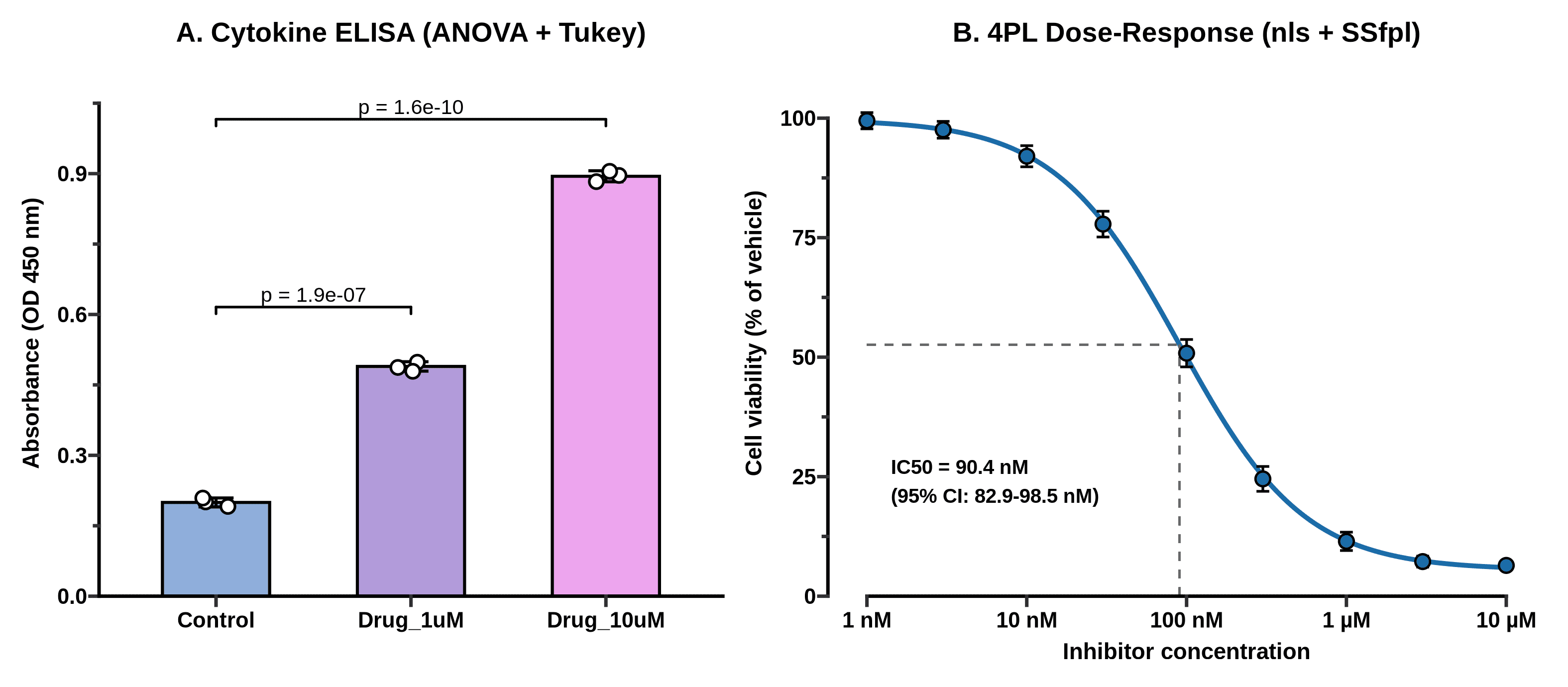
_Figure 1. Replacing GraphPad Prism in R. Left: one-way ANOVA and Tukey HSD on biological replicates from elisa_data.csv, styled with ggprism and ggsignif. Right: four-parameter logistic (4PL) dose-response curve fit with base R's nls() and SSfpl(), showing an of 90.4 nM (95% profile-likelihood CI: 82.9–98.5 nM). Output of the code above._
If you hand that PNG to a PI who has used GraphPad Prism since 2004, they will not blink. And unlike a .pzfx file, when Reviewer 2 asks you six months from now to change the palette or re-run the curve fit with the vehicle control normalized differently, you change one line and re-run the script in two seconds.
What if you want a click-and-point GUI for basic stats instead of R? Look at jamovi or JASP. Both are free, open-source desktop applications built on top of R that give you a spreadsheet interface for t-tests, ANOVAs, non-parametric tests, and regression without typing a command. They don't do 4PL pharmacology curves out of the box the way R's SSfpl() or the drc package does, but for a quick two-way ANOVA at the bench, jamovi is genuinely pleasant.
2. Replacing SnapGene: OpenCloning + ApE + pLannotate + Biopython
What you're paying now: ~$495–650/year per academic seat (or thousands for a lab group license).
SnapGene is popular for a reason: it is fast, its plasmid maps look clean, its automatic feature detection works, and its "Simulate Agarose Gel" window has saved every molecular biologist from misreading a diagnostic restriction digest at least once.
No single open-source program replaces every tab of SnapGene identically. Instead, the free stack splits SnapGene's job into four focused tools — and in a few areas, actually beats it:
- OpenCloning (MIT license, web or self-hosted Docker): As I covered in my full hands-on review of OpenCloning, this is the best tool available — free or paid — for recording how your construct was built. It simulates PCR, Gibson, Golden Gate, restriction-ligation, homologous recombination, and Gateway assemblies in the browser or via pydna, and imports SnapGene
.dnafiles with their full lineage intact. - ApE — A plasmid Editor (Free, GPL v3 since v3.1.7): Written and maintained by M. Wayne Davis in Erik Jorgensen's lab at the University of Utah, ApE is the quiet workhorse of yeast, worm, and fly genetics labs. It opens instantly on Windows, macOS, and Linux, highlights restriction sites, aligns Sanger sequencing chromatograms directly against your reference plasmid, and draws simulated restriction gels. Its interface looks like classic Tcl/Tk desktop software from the 2000s, because it is — and it never nags you for a license renewal.
- pLannotate (Free web server + open-source CLI/Docker, GPLv3): Developed in Jeffrey Barrick's lab at UT Austin, pLannotate solves the one feature people miss most when they drop SnapGene: automatic plasmid annotation from a raw sequence. Paste in an unannotated FASTA from whole-plasmid Nanopore sequencing (like a Plasmidsaurus return), and pLannotate searches Swiss-Prot, Pfam, Rfam, and SnapGene's own curated feature library to hand you back a fully annotated GenBank file and interactive map.
Biopython+dna_features_viewer(Open-source Python): When you need to screen restriction digests across a dozen constructs or generate publication-ready vector maps and diagnostic gels reproducibly from a script.
Let's run that fourth workflow right now. Using the Python environment we set up (see Python for biologists or Conda for biologists if you're new to virtual environments), install biopython, dna_features_viewer, and matplotlib:
uv pip install biopython dna_features_viewer matplotlib
Now let's fetch pUC19 (L09137.2, 2,686 bp) from NCBI, run a circular restriction batch with EcoRI, HindIII, PvuII, and BsaI, calculate the exact fragment lengths for four diagnostic digests, and plot both the circular map and a simulated 1.2% agarose gel with mass-proportional band intensity:
import urllib.request
from Bio import SeqIO
from Bio.Restriction import EcoRI, HindIII, PvuII, BsaI, RestrictionBatch
from dna_features_viewer import GraphicFeature, CircularGraphicRecord
import matplotlib.pyplot as plt

# 1. Fetch pUC19 GenBank record from NCBI (L09137.2)
url = (
    "https://eutils.ncbi.nlm.nih.gov/entrez/eutils/efetch.fcgi"
    "?db=nuccore&id=L09137.2&rettype=gbwithparts&retmode=text"
)
urllib.request.urlretrieve(url, "pUC19.gb")

record = SeqIO.read("pUC19.gb", "genbank")
print(f"Plasmid: {record.id} ({len(record.seq)} bp)")

# 2. Search restriction sites on a circular topology
rb = RestrictionBatch([EcoRI, HindIII, PvuII, BsaI])
cuts = rb.search(record.seq, linear=False)
for enzyme, sites in sorted(cuts.items(), key=lambda x: str(x[0])):
    print(f"{str(enzyme):8s}: {len(sites)} cut(s) at {sites}")

def circular_digest_sizes(seq_len, cut_positions):
    pts = sorted(cut_positions)
    if len(pts) <= 1:
        return [seq_len]
    diffs = [pts[i + 1] - pts[i] for i in range(len(pts) - 1)]
    diffs.append(seq_len - pts[-1] + pts[0])
    return sorted(diffs, reverse=True)

digests = {
    "EcoRI": circular_digest_sizes(len(record.seq), cuts[EcoRI]),
    "PvuII": circular_digest_sizes(len(record.seq), cuts[PvuII]),
    "EcoRI + PvuII": circular_digest_sizes(len(record.seq), cuts[EcoRI] + cuts[PvuII]),
    "BsaI + PvuII": circular_digest_sizes(len(record.seq), cuts[BsaI] + cuts[PvuII]),
}

print("\n--- Predicted Agarose Gel Fragments (bp) ---")
for label, frags in digests.items():
    print(f"{label:16s}: {frags} (sum = {sum(frags)} bp)")
Plasmid: L09137.2 (2686 bp)
BsaI    : 1 cut(s) at [1761]
EcoRI   : 1 cut(s) at [397]
HindIII : 1 cut(s) at [448]
PvuII   : 2 cut(s) at [309, 631]

--- Predicted Agarose Gel Fragments (bp) ---
EcoRI           : [2686] (sum = 2686 bp)
PvuII           : [2364, 322] (sum = 2686 bp)
EcoRI + PvuII   : [2364, 234, 88] (sum = 2686 bp)
BsaI + PvuII    : [1234, 1130, 322] (sum = 2686 bp)
Notice Bio.Restriction's linear=False flag. One of the classic bugs when someone tries to calculate restriction fragments in a spreadsheet is forgetting that a circular plasmid cut times produces fragments (with the wrap-around fragment spanning seq_len - last_cut + first_cut), whereas a linear amplicon cut times produces fragments. Setting linear=False handles the circular wrap-around properly.
Now render the circular feature map alongside the simulated diagnostic gel:
fig, (ax_map, ax_gel) = plt.subplots(
    1, 2, figsize=(11, 5.0), gridspec_kw={"width_ratios": [1.1, 1.0]}
)

features = [
    GraphicFeature(start=149, end=469, strand=-1, color="#4C9BE8", label="lacZα (MCS)"),
    GraphicFeature(start=853, end=1441, strand=-1, color="#F4B942", label="pMB1 ori"),
    GraphicFeature(start=1626, end=2486, strand=-1, color="#52B788", label="AmpR (bla)"),
    GraphicFeature(start=397, end=398, strand=0, color="#E63946", label="EcoRI (397)"),
    GraphicFeature(start=448, end=449, strand=0, color="#E63946", label="HindIII (448)"),
    GraphicFeature(start=309, end=310, strand=0, color="#9B5DE5", label="PvuII (309)"),
    GraphicFeature(start=631, end=632, strand=0, color="#9B5DE5", label="PvuII (631)"),
    GraphicFeature(start=1761, end=1762, strand=0, color="#E63946", label="BsaI (1761)"),
]
circ_rec = CircularGraphicRecord(sequence_length=len(record.seq), features=features, top_position=0)
circ_rec.plot(ax=ax_map, figure_width=5.2)
ax_map.set_title("A. pUC19 Map & Restriction Cuts (2,686 bp)", fontsize=12, fontweight="bold", pad=12)

ax_gel.set_facecolor("#12161F")
ladder_bp = [3000, 2000, 1500, 1000, 700, 500, 400, 300, 200, 100]
lanes = ["Ladder", "EcoRI", "PvuII", "EcoRI +\nPvuII", "BsaI +\nPvuII"]

for bp in ladder_bp:
    lw = 3.6 if bp in (1000, 3000) else 2.0
    alpha = 0.95 if bp in (1000, 3000) else 0.72
    ax_gel.plot([-0.24, 0.24], [bp, bp], color="#E8F1F5", linewidth=lw, alpha=alpha, solid_capstyle="round")
    ax_gel.text(-0.32, bp, f"{bp}", color="#CBD5E1", fontsize=8.5, ha="right", va="center", fontweight="bold")

for idx, (label, frags) in enumerate(digests.items(), start=1):
    for bp in frags:
        mass_frac = bp / len(record.seq)
        lw = 1.6 + 3.2 * mass_frac
        alpha = min(0.98, 0.45 + 0.75 * mass_frac)
        ax_gel.plot([idx - 0.24, idx + 0.24], [bp, bp], color="#70E000", linewidth=lw, alpha=alpha, solid_capstyle="round")
        ax_gel.text(idx + 0.29, bp, f"{bp}", color="#9EF01A", fontsize=8, ha="left", va="center")

ax_gel.set_yscale("log")
ax_gel.set_ylim(70, 4200)
ax_gel.set_xlim(-0.82, 4.80)
ax_gel.set_xticks(range(len(lanes)))
ax_gel.set_xticklabels(lanes, fontsize=9.5, fontweight="bold")
ax_gel.yaxis.set_visible(False)
ax_gel.set_title("B. In-Silico Diagnostic Digest Gel", fontsize=12, fontweight="bold", pad=12)

plt.tight_layout()
plt.savefig("public/static/images/fig-free-stack-plasmid-digest.png", dpi=300, facecolor="white")
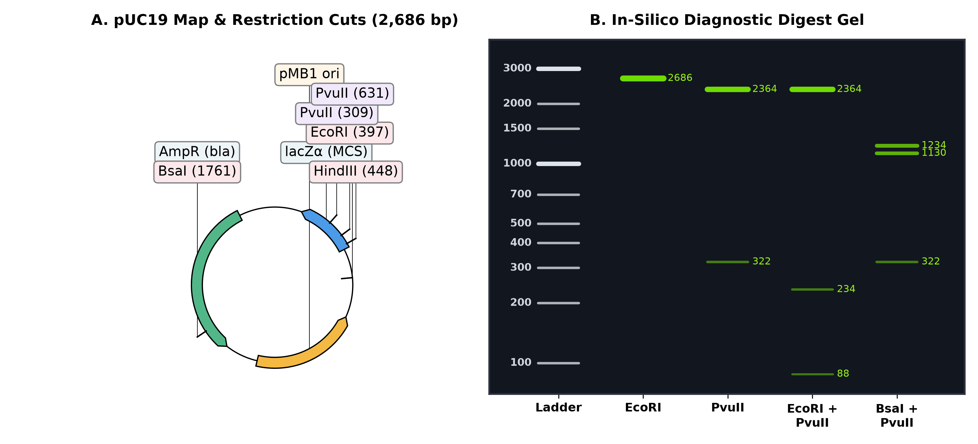
Figure 2. Replacing SnapGene's plasmid map and gel simulator in Python (Biopython + dna_features_viewer). Notice that band brightness scales with bp / total_length, reproducing why the 88 bp fragment in the EcoRI + PvuII lane is barely visible under UV transillumination unless you overload the well. Output of the code above.
If you also need primer design for cloning or diagnostic colony PCR, pair this with Primer-BLAST or Primer3Plus — covered in detail in the PCR primer design tools guide.
3. Replacing FlowJo: FlowKit (Python) and flowCore / CytoExploreR (R)
What you're paying now: ~$550–1,200+/year per seat or hardware dongle.
FlowJo is the hardest habit in a cell biology or immunology lab to break. Drawing polygon gates with a mouse on biaxial dot plots feels tactile and immediate in a way that typing gate coordinates never will.
But FlowJo has two massive problems beyond its price tag:
- Manual gating is quietly irreproducible. Give two experienced postdocs the same 20
.fcsfiles and ask them to gate live singlets and a dim fluorescence marker by hand. Their gates will drift slightly from tube to tube, and if someone loses the.wspworkspace file, you can never reconstruct the exact boundaries that produced Figure 3C. - For routine bench assays — like checking a CRISPR-EGFP knock-in, a lentiviral transduction MOI, or an Annexin V / PI viability stain — you don't need 18-color spectral compensation. You need a clean live-cell gate, a threshold gate set against your unstained or mock-transfected control, and a table of percentages that exports straight into your lab notebook.
You have two strong free options depending on your language preference:
- In R / Bioconductor:
flowCore+ggcyto+openCytoare the gold standard for scripted cytometry pipelines. And if you do want interactive mouse-driven gate drawing inside R, Dillon Hammill's CytoExploreR lets you draw gates with your cursor in an R graphics window and automatically saves them into a reproducible BioconductorGatingSet. - In Python: FlowKit (developed by Scott White and colleagues, BSD-3-Clause license) reads and writes standard FCS 2.0/3.0/3.1 files, handles fluorescence compensation matrices, provides true FlowJo-compatible logicle (biexponential) and hyperlog transforms, and imports/exports GatingML 2.0 and FlowJo 10
.wspworkspaces.
Let's run a complete FlowKit workflow on a 10,000-event FCS 3.1 file from a CRISPR-Cas9 HDR knock-in experiment where cells were edited to insert an in-frame EGFP tag and counterstained with Propidium Iodide (PI) to exclude dead cells:
import numpy as np
import flowio
import flowkit as fk
import matplotlib.pyplot as plt

# Load the FCS 3.1 file and inspect its channel metadata
sample = fk.Sample("crispr_gfp_knockin.fcs")
print(sample)
print(sample.channels[["channel_number", "pnn", "pns"]])
Sample(v3.1, crispr_gfp_knockin.fcs, 4 channels, 10000 events)
   channel_number             pnn               pns
0               1           FSC-A   Forward Scatter
1               2           SSC-A      Side Scatter
2               3          FITC-A              EGFP
3               4  PE-Texas Red-A  Propidium Iodide
Now apply a logicle transform, extract the event matrix, apply the two sequential gates (Gate 1: live cells with intact membrane, FSC-A between 75,000 and 165,000 and PI < 1,000; Gate 2: EGFP+ cells among the live population, FITC-A >= 3,000), and print the exact cell counts and percentages:
xform = fk.transforms.LogicleTransform(param_t=262144, param_w=0.5, param_m=4.5, param_a=0)
sample.apply_transform(xform)

df = sample.as_dataframe(source="raw")
df.columns = [c[0] for c in df.columns]

live_mask = (df["FSC-A"] >= 75000) & (df["FSC-A"] <= 165000) & (df["PE-Texas Red-A"] < 1000)
gfp_mask = live_mask & (df["FITC-A"] >= 3000)

pct_live = 100.0 * live_mask.sum() / len(df)
pct_gfp_of_live = 100.0 * gfp_mask.sum() / live_mask.sum()

print(f"Total events   : {len(df)}")
print(f"Live gate      : {live_mask.sum()} / {len(df)} ({pct_live:.1f}%)")
print(f"EGFP+ (of Live): {gfp_mask.sum()} / {live_mask.sum()} ({pct_gfp_of_live:.1f}%)")
Total events   : 10000
Live gate      : 8431 / 10000 (84.3%)
EGFP+ (of Live): 5227 / 8431 (62.0%)
And plot the biaxial density plot for Gate 1 alongside the gated fluorescence histogram for Gate 2:
fig, (ax1, ax2) = plt.subplots(1, 2, figsize=(10.5, 4.5))

ax1.hexbin(
    df["FSC-A"] / 1000, np.log10(df["PE-Texas Red-A"]),
    gridsize=55, cmap="viridis", mincnt=1, bins="log"
)
rect_x = [75, 165, 165, 75, 75]
rect_y = [1.0, 1.0, 3.0, 3.0, 1.0]
ax1.plot(rect_x, rect_y, color="#E63946", linewidth=2.2)
ax1.text(
    78, 2.75, f"Live cells\n{pct_live:.1f}% ({live_mask.sum():,})",
    color="#E63946", fontweight="bold", fontsize=10,
    bbox=dict(boxstyle="round,pad=0.25", facecolor="white", edgecolor="#E63946", alpha=0.9)
)
ax1.set_xlabel("Forward Scatter (FSC-A, ×10³)", fontweight="bold")
ax1.set_ylabel("log10(Propidium Iodide, PE-Texas Red-A)", fontweight="bold")
ax1.set_title("A. Gate 1: Viability (FSC-A vs PI)", fontweight="bold")
ax1.set_xlim(10, 200)
ax1.set_ylim(0.8, 5.2)

live_df = df[live_mask]
ax2.hist(np.log10(live_df["FITC-A"]), bins=65, color="#3A86FF", edgecolor="black", linewidth=0.4, alpha=0.82)
ax2.set_ylim(0, 580)
ax2.axvline(np.log10(3000), color="#E63946", linestyle="--", linewidth=2.0)
ax2.axvspan(np.log10(3000), 5.3, color="#52B788", alpha=0.18)
ax2.text(
    3.56, 515, f"EGFP+ Knock-in\n{pct_gfp_of_live:.1f}% ({gfp_mask.sum():,})",
    color="#1B4332", fontweight="bold", fontsize=10,
    bbox=dict(boxstyle="round,pad=0.3", facecolor="white", edgecolor="#52B788", alpha=0.95)
)
ax2.set_xlabel("log10(EGFP Fluorescence, FITC-A)", fontweight="bold")
ax2.set_ylabel("Cell Count (gated on Live)", fontweight="bold")
ax2.set_title("B. Gate 2: EGFP Knock-In Efficiency", fontweight="bold")
ax2.set_xlim(1.0, 5.3)

plt.tight_layout()
plt.savefig("public/static/images/fig-free-stack-flow-gating.png", dpi=300, facecolor="white")
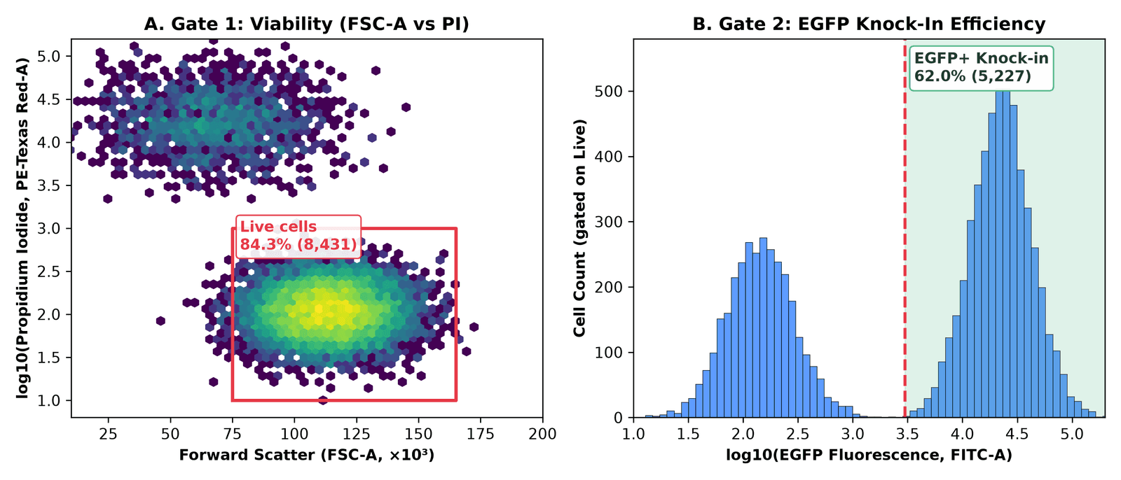
Figure 3. Scripted flow cytometry gating with Python's FlowKit. Gate 1 excludes PI-positive dead cells and low-FSC debris (retaining 8,431 of 10,000 events, 84.3%); Gate 2 quantifies EGFP+ knock-in efficiency among live cells (5,227 of 8,431 events, 62.0%). Output of the code above.
If you are running a 96-well plate of CRISPR guides on an Attune or CytoFLEX, wrapping that block in a for fcs_file in glob("*.fcs"): loop processes all 96 wells in four seconds, applies the exact same gate to every well, and writes out a CSV ready for plotting. And if you want to validate what is happening at the DNA level underneath that 62% EGFP signal, combine it with the methods in On-target CRISPR assessment: T7E1, TIDE, and amplicon NGS.
4. Replacing BioRender: NIH BioArt + Bioicons + Inkscape + CellPAINT
What you're paying now: ~$420/year per academic seat (free tier blocks high-res export, adds watermarks, and prohibits journal publication without a paid license).
BioRender's business model is clever: make the icon library so convenient during lab meetings that by the time you write your paper or thesis, redrawing your schematics feels impossible — so you pay to unlock the publication license confirmation PDF that journals ask for.
Two years ago, replacing BioRender with free tools meant cobbling together inconsistent clipart. In 2026, the open-access scientific icon ecosystem is genuinely good, provided you bookmark three specific libraries and pair them with Inkscape (the free, open-source vector editor that replaces Adobe Illustrator):
- NIH BioArt Source (Public Domain / CC BY): Released by the National Institute of Allergy and Infectious Diseases (NIAID), this is the single biggest upgrade to the free illustration stack. It provides over 2,000 professionally illustrated biomedical vector icons and brushes — lipid bilayers, viral capsids, immune cells, labware, model organisms, and signaling proteins — created by professional medical illustrators. Every asset can be downloaded as a clean SVG and edited down to individual paths in Inkscape, with zero licensing fees for journal publication or book chapters.
- Bioicons (CC0 / CC BY) and SciDraw (CC BY): Community-curated repositories containing over 2,700 vector icons covering molecular biology, neuroscience setups, behavioural arenas, and sequencing hardware. Bioicons even ships an official Inkscape extension so you can drag icons straight onto your canvas without leaving the editor.
- CellPAINT and UCSF ChimeraX: When you want your figure to show real molecular scale rather than cartoons, read our guide to CellPAINT or load your structure (or AlphaFold3 prediction) into ChimeraX. Here is a one-line ChimeraX command-bar trick that turns any PDB file into a flat-shaded, Goodsell/BioRender-style protein illustration with crisp black outlines ready to drop into an Inkscape figure:
lighting flat; graphics silhouettes true width 2; color bychain; set bgColor white
Run that in ChimeraX's command bar on Cas9 (PDB: 4OO8) or your protein of interest, export a transparent PNG (save protein_icon.png transparentBackground true supersample 3), and you have a structurally accurate icon that you own outright.
5. Bonus: replacing paid image analysis and proprietary ELNs
Two more categories quietly drain lab budgets once a group grows past a few people:
Microscopy, gels, and colony counting: Fiji + CellProfiler + QuPath
Commercial image analysis suites (Imaris, HALO, or paid Zen/NIS-Elements quantification modules) routinely cost $3,000 to $15,000+ per workstation. Meanwhile, the open-source bioimage stack is one of the greatest success stories in scientific software:
- Fiji (ImageJ2) (GPLv2+): Still the undisputed standard for Western blot densitometry, multichannel TIFF merging, scale bars, and macro automation.
- CellProfiler (BSD-3-Clause, Broad Institute): When you have 500 fluorescence microscopy fields and need to segment nuclei, measure cytoplasmic-to-nuclear translocation of a transcription factor, and export per-cell tables without hand-drawing ROIs.
- QuPath (GPLv3): Originally built for whole-slide digital pathology and spatial transcriptomics/immunofluorescence, QuPath handles massive pyramidal
.ome.tiffand.svsimages that crash Fiji, with built-in StarDist and Cellpose deep-learning segmentation plugins.
Electronic lab notebooks (ELNs): eLabFTW and BenchOS
Benchling's academic tier is free, which makes it the default in many molecular biology departments — right up until a spin-out company forms, an industry collaboration requires on-premise data residency, or you try to export five years of interconnected notebook entries and registry links.
- eLabFTW (AGPLv3): The mature, battle-tested open-source ELN used by hundreds of academic labs and core facilities. It runs in Docker, includes a proper inventory/database for plasmids, antibodies, and cell lines, supports RFC 3161 trusted timestamps for IP protection, and integrates directly with OpenCloning so your plasmid maps render inline inside your experiment notes.
- BenchOS (AGPLv3): A newer, molecular- and structural-biology-first self-hosted lab operating system from the Farnung Lab at Harvard Medical School. I installed and tested it in my hands-on BenchOS review — it is early-stage (
v0.1.0), but its built-in cryo-EM grid tracking and molecular biology calculators are worth watching.
The master comparison table
| Lab workflow | Commercial incumbent (typical academic cost) | Free & open-source replacement | License | Difficulty to switch |
|---|---|---|---|---|
| Lab stats & bar/dot plots | GraphPad Prism (~$310–550/yr) | R + ggplot2 + ggprism + ggsignif (or jamovi for GUI) | GPL / MIT | Low–Medium |
| 4PL dose-response / IC50 | GraphPad Prism (~$310–550/yr) | R base nls() + SSfpl() (or drc package) | GPL | Medium |
| Plasmid viewing & Sanger trace alignment | SnapGene (~$495–650/yr) | ApE (A plasmid Editor) | GPLv3 | Very Low |
| Cloning lineage & assembly simulation | SnapGene / Benchling | OpenCloning + pydna | MIT / BSD | Low |
| Auto-annotating raw plasmid FASTAs | SnapGene | pLannotate (web or Docker) | GPLv3 | Very Low |
| Batch digest maps & gel simulation | SnapGene | Biopython + dna_features_viewer | BSD / MIT | Medium |
| Flow cytometry gating (2–6 colors) | FlowJo (~$550–1,200/yr) | FlowKit (Python) or flowCore + CytoExploreR (R) | BSD / Artistic-2.0 | Medium–High |
| Pathway schematics & graphical abstracts | BioRender (~$420/yr) | NIH BioArt + Bioicons + Inkscape + CellPAINT | Public Domain / CC0 / GPL | Low–Medium |
| Microscopy & Western quantification | Imaris / HALO ($3,000+/yr) | Fiji (ImageJ), CellProfiler, QuPath | GPL / BSD | Low |
| Electronic lab notebook & inventory | Benchling (paid tiers) / LabArchives | eLabFTW (or BenchOS) | AGPLv3 | Medium (needs Docker) |
The real talk: where the free stack still loses
I champion open-source tools on this blog, and I use the stack above every week. But pretending there are no trade-offs is how people get burned and go right back to paying for subscriptions. Here is where the commercial tools are still genuinely ahead:
- High-dimensional (16–40 color) interactive flow cytometry exploration. If you are an immunologist building a 28-color spectral flow panel on an Aurora, tweaking compensation matrices interactively by dragging sliders, and exploring rare T-cell subsets in real time, FlowJo (or OMIQ) is still faster than writing
FlowKitorflowCorescripts. Scripted gating shines once your panel is fixed and you want to process 50 tubes identically; it is clunky when you don't yet know where the populations sit. - Speed of throwing together a last-minute slide in BioRender. Pulling SVGs from
NIH BioArtandBioiconsinto Inkscape produces cleaner, license-free figures that you own forever. It also takes 45 minutes instead of 15 minutes the first few times you do it, because you don't have BioRender's pre-styled membrane brushes and one-click callout templates under one search bar. - SnapGene's polish for interactive primer-walking and visual history. Combining
ApE(for daily desktop viewing and trace alignment),pLannotate(for auto-annotating Nanopore plasmid sequences), andOpenCloning(for cloning lineage and Gibson/Golden Gate simulation) covers everything SnapGene does. Splitting one habit across three tools still takes a week of muscle-memory adjustment. - Someone has to back up self-hosted servers. Tools like
eLabFTW,BenchOS, and self-hostedOpenCloningare free of subscription fees, not free of responsibility. If you run an ELN in Docker on an old workstation under a bench and the hard drive dies without an automated off-site backup, there is no vendor support line to rescue your lab notebooks.
My recommendation: how to actually migrate without a lab mutiny
If you walk into lab meeting on Monday and announce that everyone is deleting Prism, SnapGene, and BioRender cold turkey, your lab mates will stage a coup by Wednesday.
Do it in this order instead:
- Week 1 (Zero friction): Bookmark NIH BioArt Source and Bioicons, install Inkscape, and install ApE alongside pLannotate. Neither requires writing a line of code, and any undergraduate or rotating student can use them immediately without asking the lab manager for a license seat.
- Week 2 (Cloning provenance): Design your next two constructs in OpenCloning and save the
.jsonhistory file alongside your sequence map. - Week 3 (Retire Prism for your next figure): Take the R script in Section 1 above — or start from Post 1 of the R for Biologists series — and build your next ELISA, qPCR, or viability dose-response figure with
ggplot2andggprism. Once you have that single.Rfile saved in your project folder, every future assay is a five-minute copy-and-edit job. - Week 4 (Automate repetitive assays): If your lab runs recurring flow cytometry readouts (like CRISPR reporter screens or viral titers) or CRISPR editing validation, move those into reproducible scripts (
FlowKitin Python, or the NGS pipelines covered in the CRISPR from Bench to Analysis series and the CRISPR from Bench to Analysis book).
You don't have to be a computational biologist to own your own tools. Every script and file format in this stack is plain text, open standard, and free — which means your analysis still belongs to you long after your current license key expires.
Which paid piece of lab software would you most like to get rid of — or which free alternative has saved your lab budget? Drop a comment below.
Resources
| Tool / Package | Category | License | Link |
|---|---|---|---|
| ggprism | Prism-styled themes & axes for ggplot2 | GPL-3 | csdaw.github.io/ggprism |
| ggsignif | Significance brackets for ggplot2 | GPL-3 | cran.r-project.org/package=ggsignif |
| patchwork | Multi-panel figure composition in R | MIT | patchwork.data-imaginist.com |
| jamovi | Free GUI statistical spreadsheet built on R | AGPLv3 | jamovi.org |
| OpenCloning | Open-source cloning simulation & lineage app | MIT | opencloning.org |
| pydna | Python cloning & assembly simulation library | BSD-3-Clause | github.com/pydna-group/pydna |
| ApE (A plasmid Editor) | Desktop plasmid editor & Sanger aligner | GPLv3 | jorgensen.biology.utah.edu/wayned/ape |
| pLannotate | Automatic plasmid feature annotation | GPLv3 | plannotate.barricklab.org |
| Biopython | Sequence & restriction analysis in Python | Biopython / BSD | biopython.org |
| dna_features_viewer | Linear & circular sequence map plotting | MIT | github.com/Edinburgh-Genome-Foundry/DnaFeaturesViewer |
| FlowKit | FCS 3.1 parsing, logicle transforms & gating in Python | BSD-3-Clause | flowkit.readthedocs.io |
| flowCore / ggcyto | Bioconductor flow cytometry infrastructure in R | Artistic-2.0 | bioconductor.org/packages/flowCore |
| CytoExploreR | Interactive mouse-driven flow gating in R | GPL-3 | dillonhammill.github.io/CytoExploreR |
| NIH BioArt Source | 2,000+ free biomedical SVG icons & brushes | Public Domain / CC BY | bioart.niaid.nih.gov |
| Bioicons | 2,700+ open-source science vector icons | CC0 / CC BY | bioicons.com |
| SciDraw | Community-contributed scientific schematics | CC BY | scidraw.io |
| Inkscape | Open-source vector graphics editor | GPLv2+ | inkscape.org |
| CellPAINT | Mesoscale molecular illustration tool | Open source | ccsb.scripps.edu/cellpaint |
| UCSF ChimeraX | 3D molecular visualization & flat-lit rendering | Free for academic use | rbvi.ucsf.edu/chimerax |
| Fiji (ImageJ) | Scientific image processing & densitometry | GPLv2+ | fiji.sc |
| CellProfiler | Automated high-content cell image analysis | BSD-3-Clause | cellprofiler.org |
| QuPath | Whole-slide bioimage analysis & segmentation | GPLv3 | qupath.github.io |
| eLabFTW | Self-hosted open-source electronic lab notebook | AGPLv3 | elabftw.net |
| BenchOS | Self-hosted molecular & structural biology ELN | AGPLv3 | github.com/farnunglab/BenchOS |
Keep reading
OpenCloning: the free, open-source tool that documents how your plasmid was actually built
A free, MIT-licensed web app that treats your cloning history — not just the final map — as the thing worth saving. I ran it self-hosted, cloned URA3 into pUC19 from a Python script, and looked hard at where it falls short of SnapGene and Benchling.
BenchOS: a free, self-hosted lab operating system for molecular and structural biology
A Harvard structural biology lab just open-sourced the software it runs its own bench on — notebook, registry, cryo-EM grid tracking, and an AI agent, all self-hosted under AGPL. I installed it and ran it. Here is what actually works, and what you should know before trusting it with your lab records.
CellPAINT: The Free Tool That Turns Molecular Biology Into Art
An in-depth look at CellPAINT — the free, scientifically accurate molecular painting tool from Scripps — and how it compares to BioRender, ChimeraX, PyMOL, and other illustration platforms.