- Published on
- 23 min read
How to analyze qPCR data: the ΔΔCt method step by step (by hand, in a spreadsheet, and in R)
- Authors

- Name
- BioTech Bench
Table of contents
- What you'll learn
- What a Ct value tells you
- The ΔΔCt method in four steps
- The same calculation in a spreadsheet
- The same calculation in R
- Which numbers get the statistics?
- When ΔΔCt is not valid: efficiency and the Pfaffl correction
- Is your reference gene behaving?
- Common mistakes
- The real talk: what this method can't do
- What I'd actually do
- Resources
The run finished twenty minutes ago. The amplification curves look clean, the melt curves have one peak each, and the instrument software has exported a spreadsheet with a column called "Ct" (or "Cq", depending on the machine). Now somebody needs to turn those numbers into the bar chart for lab meeting, and that somebody is you.
Let me guess how the next hour goes. You search for "delta delta Ct", find a formula with a superscript in it, open the spreadsheet a former postdoc left on the shared drive, paste your values over theirs, and hope the cell references still point where they should. A number comes out. You're not completely sure what it means or whether the error bars are right.
I've done exactly that, and I've also been the person who later found the broken cell reference. So this post walks through the whole calculation three times: once by hand so you can see every subtraction, once in a spreadsheet you can download, and once in R so you never have to paste over anyone's old file again. All three give the same answer, and I'll show you that they do.
What you'll learn
- What a Ct value measures, and why a difference of one cycle means roughly a two-fold difference
- The four steps of the ΔΔCt method, worked by hand on real numbers
- How to do the same calculation in a spreadsheet (template included) and in R with
dplyr - Which numbers to plot, which numbers to run statistics on, and why they aren't the same ones
- When the ΔΔCt shortcut isn't valid, and what the Pfaffl correction does about it
- The common mistakes: averaging fold changes, counting wells as replicates, trusting one reference gene
What a Ct value tells you
During qPCR, the amount of product roughly doubles every cycle, and a fluorescent dye or probe reports how much product there is. The Ct (cycle threshold) is the cycle at which the fluorescence of a well crosses a fixed threshold. A sample that started with a lot of template crosses early and gets a low Ct. A sample that started with very little crosses late and gets a high Ct.
Two things follow from that, and everything else in this post builds on them:
- Ct runs backwards. Lower Ct means more starting material. This trips up everyone at least once.
- Ct is a log scale. If product doubles each cycle, a sample that crosses one cycle earlier started with about twice as much template. Two cycles earlier is about four times as much. Ten-fold is about 3.3 cycles.
A quick note on names: the MIQE guidelines recommend Cq (quantification cycle) as the standard term, and some instruments say Cp. They all mean the same thing. I'll say Ct here because that's what the method is called and what most people type into a search box.
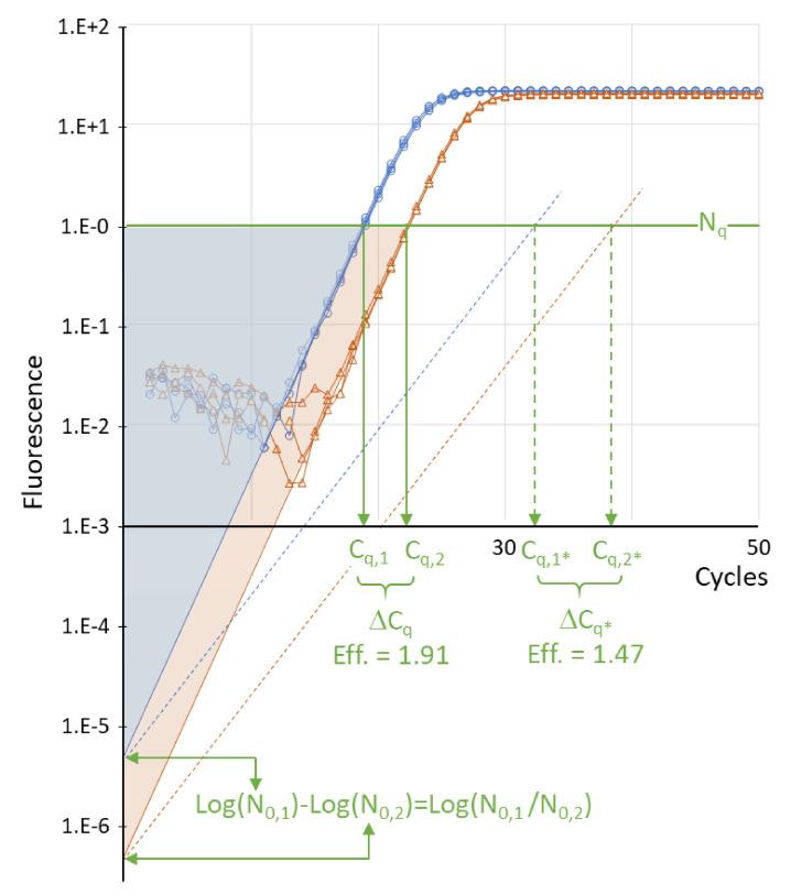
Figure 1. Where Ct comes from. Two sets of reactions with about a ten-fold difference in starting template (blue and orange) cross the threshold (green line) a few cycles apart. That gap is the ΔCt. The dotted lines show the same two samples amplified by a less efficient assay: both cross later, and the gap between them is wider, which is why efficiency matters later in this post. Adapted from Ruiz-Villalba A, Ruijter JM, van den Hoff MJB (2021). Use and misuse of Cq in qPCR data analysis and reporting. _Life, 11:496. doi:10.3390/life11060496, under CC BY 4.0._
A raw Ct on its own doesn't tell you about expression, though. If you loaded a bit more cDNA into one well, every gene in that well crosses earlier. That's the problem the ΔΔCt method solves, with two subtractions.
The ΔΔCt method in four steps
The method comes from Livak and Schmittgen's 2001 paper, which is one of the most cited papers in molecular biology for a reason: almost every relative expression figure you've seen uses it.
- Average your technical replicates so each biological sample has one Ct per gene.
- ΔCt = Ct of target gene − Ct of reference gene, within each sample. This corrects for how much cDNA went into the well.
- ΔΔCt = ΔCt of the sample − mean ΔCt of the control group. This expresses every sample relative to your control (the "calibrator").
- Fold change = 2^(−ΔΔCt). The minus sign flips the backwards Ct scale, and the 2 turns cycles back into amounts.
Because of that last step, you can read ΔΔCt values almost directly:
| ΔΔCt | Fold change vs control | In words |
|---|---|---|
| 0 | 1 | No change |
| −1 | 2 | Doubled |
| −2 | 4 | Four times higher |
| −3.3 | about 10 | Ten times higher |
| +1 | 0.5 | Halved |
The example dataset
I'll use the same small dataset as the R for Biologists series so you can follow along: cells treated with two doses of LPS, three biological replicates per group, with IL6, TNF and IL10 as targets and GAPDH as the reference gene. Download qpcr_data.csv if you want to reproduce every number below.
It's a teaching dataset, built to look like a typical cytokine induction experiment, so don't cite the biology. The arithmetic is what matters here.
Working one sample by hand
Take IL6 in the three control samples and one sample from the high-dose group.
| Sample | Group | IL6 Ct | GAPDH Ct | ΔCt (IL6 − GAPDH) |
|---|---|---|---|---|
| S01 | Control | 30.75 | 21.15 | 9.60 |
| S02 | Control | 31.28 | 20.87 | 10.41 |
| S03 | Control | 30.52 | 21.38 | 9.14 |
| S07 | LPS 10 ng | 23.81 | 21.02 | 2.79 |
The mean ΔCt of the control group is (9.60 + 10.41 + 9.14) / 3 = 9.72. That's the calibrator.
For sample S07:
- ΔΔCt = 2.79 − 9.72 = −6.93
- Fold change = 2^(6.93) = about 122
So IL6 in that sample is roughly 122 times higher than the control average. Notice what GAPDH did: almost nothing. It sits around Ct 21 in every sample, which is exactly what you want from a reference gene. All of the movement is in IL6, which dropped about seven cycles.
That's the entire method. Everything from here on is doing it for many samples without making a mistake.
The same calculation in a spreadsheet
Here's the honest answer about spreadsheets: they're fine for this. The calculation is three formulas. What goes wrong is never the math, it's the pasting, the dragging, and the reference that silently points at the wrong row.
With sample names in column A, groups in B, reference Ct in C and target Ct in D, starting at row 2, and the three control samples in rows 2 to 4:
| Cell | Formula | What it does |
|---|---|---|
| E2 | =D2-C2 | ΔCt for that sample |
| E13 | =AVERAGE(E2:E4) | Mean ΔCt of the control group (calibrator) |
| F2 | =E2-$E$13 | ΔΔCt (the $ signs lock the calibrator) |
| G2 | =2^(-F2) | Fold change for that sample |
| B16 | =AVERAGE(F2:F4) | Mean ΔΔCt for a group |
| C16 | =STDEV(F2:F4) | SD of ΔΔCt for a group |
| D16 | =2^(-B16) | Group fold change |
| E16 | =2^(-(B16+C16)) | Lower end of the error bar |
| F16 | =2^(-(B16-C16)) | Upper end of the error bar |
Drag E2, F2 and G2 down for the rest of your samples. The dollar signs in $E$13 are the part people forget, and without them the calibrator slides down a row with every sample.
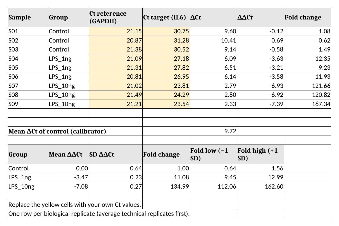
Figure 2. The filled-in template for IL6. Yellow cells are the only ones you type into. The group fold changes at the bottom (1.00, 11.08 and 134.99) are the numbers to check against the R output below. Rendered from my own template in LibreOffice Calc.
Download the template (qpcr-ddct-template.xlsx). It opens in Excel, LibreOffice Calc and Google Sheets. Replace the yellow cells with your own Ct values, one row per biological replicate.
Look closely at how the error bars are built, because it's the step most templates get wrong. The mean and SD are calculated on the ΔΔCt values, and only then converted to fold change. That gives asymmetric error bars (112 to 163 around 135), which is correct for data that lives on a log scale. More on that in the mistakes section.
The same calculation in R
If you run qPCR every week, a script beats a template. You point it at a new file and get the same analysis every time, with nothing to drag. If you've never used R, the first post in the R series gets you set up; if you have, this is about twenty lines.
library(readr)
library(dplyr)
library(tidyr)
library(ggplot2)
Load the data and set the group order so Control comes first:
qpcr <- read_csv("qpcr_data.csv", show_col_types = FALSE) |>
  mutate(group = factor(group, levels = c("Control", "LPS_1ng", "LPS_10ng")))

qpcr |>
  select(sample_id, group, GAPDH_ct, IL6_ct, TNF_ct, IL10_ct)
# A tibble: 9 × 6
  sample_id group    GAPDH_ct IL6_ct TNF_ct IL10_ct
  <chr>     <fct>       <dbl>  <dbl>  <dbl>   <dbl>
1 S01       Control      21.2   30.8   29.5    31.9
2 S02       Control      20.9   31.3   30.1    32.4
3 S03       Control      21.4   30.5   29.8    31.7
4 S04       LPS_1ng      21.1   27.2   26.9    29.3
5 S05       LPS_1ng      21.3   27.8   27.4    29.9
6 S06       LPS_1ng      20.8   27.0   27.1    28.9
7 S07       LPS_10ng     21.0   23.8   24.2    27.1
8 S08       LPS_10ng     21.5   24.3   24.7    27.6
9 S09       LPS_10ng     21.2   23.5   23.9    26.8
Each row is one biological replicate with one Ct per gene. (The tibble display rounds to three significant figures; the full values are still there.) If your export has technical replicates as separate rows, average them first. The dplyr post shows how with group_by() and summarise().
Step 1: ΔCt
Reshape so each target gene gets its own row, then subtract the reference:
dct <- qpcr |>
  select(sample_id, group, GAPDH_ct, IL6_ct, TNF_ct, IL10_ct) |>
  pivot_longer(c(IL6_ct, TNF_ct, IL10_ct), names_to = "gene", values_to = "ct") |>
  mutate(
    gene = sub("_ct", "", gene),
    dct  = ct - GAPDH_ct
  )

head(dct)
# A tibble: 6 × 6
  sample_id group   GAPDH_ct gene     ct   dct
  <chr>     <fct>      <dbl> <chr> <dbl> <dbl>
1 S01       Control     21.2 IL6    30.8  9.6
2 S01       Control     21.2 TNF    29.5  8.37
3 S01       Control     21.2 IL10   31.9 10.8
4 S02       Control     20.9 IL6    31.3 10.4
5 S02       Control     20.9 TNF    30.1  9.24
6 S02       Control     20.9 IL10   32.4 11.5
The first row is the 9.60 from the hand calculation.
Step 2: ΔΔCt and fold change
group_by(gene) makes sure each gene is compared with its own control mean:
ddct <- dct |>
  group_by(gene) |>
  mutate(
    ddct = dct - mean(dct[group == "Control"]),
    fold = 2^(-ddct)
  ) |>
  ungroup()

ddct |>
  filter(gene == "IL6") |>
  select(sample_id, group, dct, ddct, fold)
# A tibble: 9 × 5
  sample_id group      dct   ddct    fold
  <chr>     <fct>    <dbl>  <dbl>   <dbl>
1 S01       Control   9.6  -0.117   1.08
2 S02       Control  10.4   0.693   0.618
3 S03       Control   9.14 -0.577   1.49
4 S04       LPS_1ng   6.09 -3.63   12.4
5 S05       LPS_1ng   6.51 -3.21    9.23
6 S06       LPS_1ng   6.14 -3.58   11.9
7 S07       LPS_10ng  2.79 -6.93  122.
8 S08       LPS_10ng  2.8  -6.92  121.
9 S09       LPS_10ng  2.33 -7.39  167.
Sample S07 comes out at −6.93 and 122-fold, the same as by hand. Also look at the control rows: they aren't all exactly 1. They scatter from 0.62 to 1.49, because individual controls differ from the control average. That scatter is real biological variation, and you should show it rather than hide it behind a flat bar at 1.
Step 3: summarize per group
fold_summary <- ddct |>
  group_by(gene, group) |>
  summarise(
    mean_ddct = mean(ddct),
    sd_ddct   = sd(ddct),
    fold      = 2^(-mean_ddct),
    fold_low  = 2^(-(mean_ddct + sd_ddct)),
    fold_high = 2^(-(mean_ddct - sd_ddct)),
    .groups = "drop"
  )

fold_summary |>
  mutate(across(where(is.numeric), \(x) round(x, 2)))
# A tibble: 9 × 7
  gene  group    mean_ddct sd_ddct   fold fold_low fold_high
  <chr> <fct>        <dbl>   <dbl>  <dbl>    <dbl>     <dbl>
1 IL10  Control       0       0.63   1        0.65      1.55
2 IL10  LPS_1ng      -2.57    0.23   5.95     5.07      6.98
3 IL10  LPS_10ng     -4.94    0.29  30.6     25.1      37.3
4 IL6   Control       0       0.64   1        0.64      1.56
5 IL6   LPS_1ng      -3.47    0.23  11.1      9.45     13.0
6 IL6   LPS_10ng     -7.08    0.27 135.     112.      163.
7 TNF   Control       0       0.48   1        0.72      1.4
8 TNF   LPS_1ng      -2.6     0.23   6.06     5.17      7.11
9 TNF   LPS_10ng     -5.66    0.28  50.6     41.8      61.2
IL6 goes up about 11-fold at the low dose and 135-fold at the high dose. Those are the same 11.08 and 134.99 as in the spreadsheet, so the three routes agree.
Step 4: plot it
Fold changes belong on a log axis, and with three replicates per group there's no reason not to show every point:
p <- ggplot(ddct, aes(x = group, y = fold)) +
  geom_hline(yintercept = 1, linetype = "dashed", colour = "grey50") +
  geom_point(size = 2.5, alpha = 0.7,
             position = position_jitter(width = 0.08, height = 0, seed = 1)) +
  geom_point(data = fold_summary, shape = 95, size = 12, colour = "#d1495b") +
  scale_y_continuous(trans = "log2", breaks = c(0.5, 1, 2, 4, 8, 16, 32, 64, 128, 256)) +
  facet_wrap(~ gene) +
  labs(x = NULL, y = "Fold change vs control (log2 scale)") +
  theme_bw(base_size = 13) +
  theme(axis.text.x = element_text(angle = 30, hjust = 1))

ggsave("fig-qpcr-ddct-fold-change.png", p, width = 8, height = 4.5, dpi = 200)
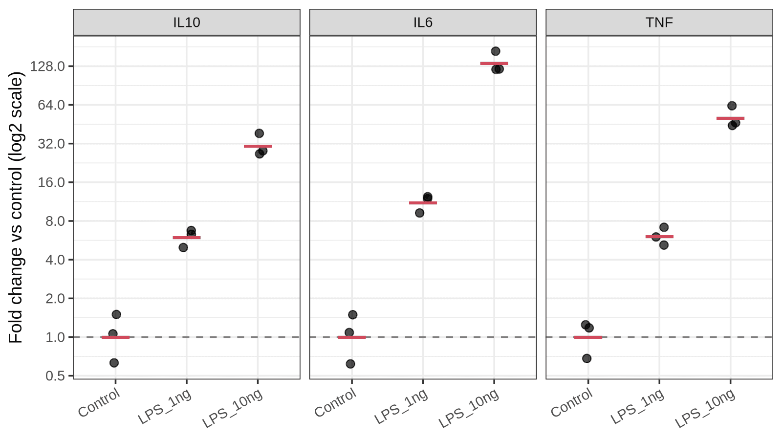
Figure 3. Fold change for the three cytokine genes. Each black point is one biological replicate, the red bar is the group fold change, and the dashed line marks no change. On a log2 axis, each gridline is one doubling, so equal distances mean equal fold differences. Output of the code above.
On a linear axis the 135-fold bar would flatten everything else into the floor, and a gene that halved would be nearly invisible next to one that doubled. The log axis treats up and down fairly.
Which numbers get the statistics?
This is the question I get asked most, and the answer surprises people: run your statistics on the ΔCt values, not on the fold changes.
Fold changes are skewed. They're squeezed between 0 and 1 for decreases and stretch out to infinity for increases, so they break the assumptions of a t-test or ANOVA. ΔCt values are on a log scale already and behave much better. The p-value you get from ΔCt is the one that goes on your figure of fold changes.
For two groups, a t-test on the IL6 ΔCt values:
il6 <- ddct |> filter(gene == "IL6")

t.test(dct ~ group, data = filter(il6, group != "LPS_1ng"))
	Welch Two Sample t-test

data:  dct by group
t = 17.591, df = 2.677, p-value = 0.0007643
alternative hypothesis: true difference in means between group Control and group LPS_10ng is not equal to 0
95 percent confidence interval:
 5.704380 8.448953
sample estimates:
 mean in group Control mean in group LPS_10ng
              9.716667               2.640000
The difference in means is 9.72 − 2.64 = 7.08 cycles, which is the ΔΔCt from the summary table with the sign flipped. The test and the fold change are describing the same quantity.
With three groups, use a one-way ANOVA followed by a post-hoc test instead of a pile of t-tests:
il6_aov <- aov(dct ~ group, data = il6)
summary(il6_aov)
TukeyHSD(il6_aov)
            Df Sum Sq Mean Sq F value   Pr(>F)
group        2  75.13   37.56   209.4 2.82e-06 ***
Residuals    6   1.08    0.18
---
Signif. codes:  0 ‘***’ 0.001 ‘**’ 0.01 ‘*’ 0.05 ‘.’ 0.1 ‘ ’ 1
  Tukey multiple comparisons of means
    95% family-wise confidence level

Fit: aov(formula = dct ~ group, data = il6)

$group
                      diff       lwr       upr     p adj
LPS_1ng-Control  -3.470000 -4.531076 -2.408924 0.0001400
LPS_10ng-Control -7.076667 -8.137742 -6.015591 0.0000021
LPS_10ng-LPS_1ng -3.606667 -4.667742 -2.545591 0.0001123
All three comparisons are significant. I'm not going to explain t-tests and ANOVA from scratch here, because the t-test and ANOVA post does that properly, including why technical replicates don't count toward your n.
When ΔΔCt is not valid: efficiency and the Pfaffl correction
Now the big "but". The 2 in 2^(−ΔΔCt) assumes that both primer pairs double the product every cycle, which is to say that both assays run at 100% amplification efficiency. Real assays usually land somewhere between 90% and 105%, and a poorly designed primer pair can be much worse.
You measure efficiency with a standard curve: run a dilution series of template (five 10-fold or 4-fold steps is typical), plot Ct against log10 of the input, and take the slope. Efficiency is 10^(−1/slope). A slope of −3.32 gives an amplification factor of 2.00 (100%), and a slope of −3.58 gives about 1.90 (90%).
If the target and reference assays have different efficiencies, the Pfaffl method (2001) replaces the 2 with each assay's own amplification factor:
- Ratio = E_target^(Ct target, control − Ct target, sample) / E_ref^(Ct ref, control − Ct ref, sample)
My example dataset has no standard curve, so I can't tell you what the real efficiencies are, and I'm not going to make them up. What I can do is show how much it would matter. Suppose the IL6 assay ran at 90% (factor 1.90) and GAPDH at 100% (factor 2.00). Those two numbers are assumptions for illustration only:
means <- qpcr |>
  group_by(group) |>
  summarise(il6 = mean(IL6_ct), gapdh = mean(GAPDH_ct))

ctrl <- filter(means, group == "Control")
lps  <- filter(means, group == "LPS_10ng")

E_target <- 1.90   # assumed: 90% efficiency for the IL6 assay
E_ref    <- 2.00   # assumed: 100% efficiency for the GAPDH assay

pfaffl <- E_target^(ctrl$il6 - lps$il6) / E_ref^(ctrl$gapdh - lps$gapdh)
livak  <- 2^(ctrl$il6 - lps$il6) / 2^(ctrl$gapdh - lps$gapdh)

c(livak = livak, pfaffl = pfaffl)
    livak    pfaffl
134.98606  94.41097
With both factors set to 2, the formula returns the same 135-fold as before, as it should. With a 90% efficient target assay, the same Ct values mean a 94-fold change. In other words, plain ΔΔCt would overstate the change by about 43% because of a ten-point efficiency gap, and the error grows with the size of the Ct difference: a 7-cycle shift is hit much harder than a 1-cycle shift.
My rule of thumb: if both assays are within 90–110% and within a few points of each other, ΔΔCt is fine and nobody will argue. If they aren't, either redesign the primers (the primer design post covers the rules) or use Pfaffl and report the efficiencies.
Is your reference gene behaving?
The whole method leans on the reference gene not changing with treatment. That's an assumption, and you can check it in one line:
qpcr |>
  group_by(group) |>
  summarise(gapdh = mean(GAPDH_ct), actb = mean(ACTB_ct))
# A tibble: 3 × 3
  group    gapdh  actb
  <fct>    <dbl> <dbl>
1 Control   21.1  19.9
2 LPS_1ng   21.1  20.1
3 LPS_10ng  21.2  20.0
Both reference genes stay within about 0.2 cycles across groups here, which is what you want to see. If your reference gene shifts by a full cycle between control and treated, your fold changes are off by a factor of two before you've started, and no formula fixes that.
GAPDH and ACTB are popular mostly out of habit. Both are known to change under some conditions (hypoxia, serum starvation, differentiation, to name three). Vandesompele and colleagues showed back in 2002 that normalizing to a single reference gene can introduce large errors, and recommended the geometric mean of several validated ones. Since Ct is a log scale, the geometric mean of the quantities is just the ordinary average of the Ct values:
qpcr |>
  mutate(
    ref_ct = (GAPDH_ct + ACTB_ct) / 2,
    dct_gapdh = IL6_ct - GAPDH_ct,
    dct_two   = IL6_ct - ref_ct
  ) |>
  group_by(group) |>
  summarise(dct_gapdh = mean(dct_gapdh), dct_two = mean(dct_two)) |>
  mutate(
    fold_gapdh = 2^(-(dct_gapdh - dct_gapdh[group == "Control"])),
    fold_two   = 2^(-(dct_two - dct_two[group == "Control"]))
  )
# A tibble: 3 × 5
  group    dct_gapdh dct_two fold_gapdh fold_two
  <fct>        <dbl>   <dbl>      <dbl>    <dbl>
1 Control       9.72   10.3         1        1
2 LPS_1ng       6.25    6.75       11.1     12.0
3 LPS_10ng      2.64    3.28      135.     133.
Using both reference genes moves the IL6 fold changes from 11.1 to 12.0 and from 135 to 133. When two references agree this well, you can trust the result more than either one alone. When they disagree, you've learned something important before a reviewer did.
Common mistakes
Averaging fold changes instead of ΔΔCt values. Convert to fold change last. If you average the per-sample fold changes, large values pull the mean upward:
il6 |>
  filter(group == "LPS_10ng") |>
  summarise(
    mean_of_folds     = mean(fold),
    fold_of_mean_ddct = 2^(-mean(ddct))
  )
# A tibble: 1 × 2
  mean_of_folds fold_of_mean_ddct
          <dbl>             <dbl>
1          137.              135.
Here the gap is small (137 vs 135) because the three replicates are tight. With noisier replicates it grows quickly, and it always errs in the direction of a bigger effect.
Symmetric error bars on fold changes. A mean ± SD calculated on fold changes can dip below zero, which is nonsense for a ratio. Calculate the SD on ΔΔCt and convert the ends, as in the summary table above, or plot on a log axis.
Treating wells as replicates. Three wells from one cDNA prep measure your pipetting. Your n is the number of independent biological samples.
Subtracting the wrong way round. ΔCt is target minus reference, and ΔΔCt is sample minus control. Flip either one and upregulated genes come out as downregulated. A quick sanity check: a gene with a lower Ct in treated samples must end up with a fold change above 1.
Trusting very late Ct values. Past roughly cycle 35 you're often amplifying a handful of template molecules, where chance alone decides whether a well gets three copies or eight. Replicates scatter widely and fold changes built on them are fragile. Check your no-template controls and treat those results with suspicion.
Pairing Ct values from different runs. Target and reference for the same sample should come from the same cDNA and ideally the same plate. If a comparison has to span plates, include a shared calibrator sample on each one.
Changing the calibrator between figures. Pick the control group once. Fold changes relative to different calibrators can't be compared.
The real talk: what this method can't do
- It gives relative numbers only. A 135-fold increase says nothing about how many transcripts there are. A gene going from 1 copy to 135 copies per cell and one going from 100 to 13,500 look identical. For copy numbers you need absolute quantification with a standard curve, or digital PCR.
- It assumes efficiency, and most people never check. Everything in the Pfaffl section applies to every ΔΔCt figure ever published without reported efficiencies. Bigger Ct differences carry bigger errors.
- It's only as good as the reference gene. If the treatment moves your reference gene, the method faithfully produces the wrong answer with tight error bars.
- Fold changes from a control near the detection limit are shaky. If the control Ct is 36 and the treated Ct is 28, the "256-fold induction" rests mostly on a noisy baseline.
- Three replicates is three replicates. The p-values above are small because the example data are clean. Real experiments with n = 3 often aren't, and no analysis method rescues an underpowered design.
- mRNA is not protein. A fold change in transcript is a reason to look at the protein, not evidence about it.
The MIQE guidelines (2009, revised as MIQE 2.0 in 2025) list what to report so someone else can judge all of this: primer sequences, efficiencies, reference gene validation, and how Ct values were determined. They're worth reading once before you write your methods section.
What I'd actually do
For a routine experiment with validated primers, I'd use plain ΔΔCt and not feel bad about it. I'd run a standard curve once for every new primer pair, write the efficiency in my notebook, and only reach for Pfaffl when an assay falls outside 90–110% and I can't redesign it.
I'd use two reference genes from the start. It costs a few extra wells and it's the cheapest insurance in the whole workflow.
And I'd move the calculation into a script sooner than feels necessary. The spreadsheet template above is fine for a one-off, and I made it so you'd have a clean one. But the third time you paste new data over old data, you're one misplaced row away from a wrong figure, and a script doesn't have rows to misplace. The complete R workflow post takes this same dataset from raw file to finished figure if you want the longer version.
How do you analyze your qPCR data: the instrument software, a spreadsheet handed down through the lab, or a script? And has a reference gene ever let you down? Drop a comment below.
Resources
| Resource | What it is | Link |
|---|---|---|
| qpcr_data.csv | Example dataset used in this post | Download |
| qpcr-ddct-template.xlsx | Spreadsheet template with the ΔΔCt formulas | Download |
| Livak & Schmittgen (2001) | The original 2^(−ΔΔCt) paper, Methods 25:402–408 | doi:10.1006/meth.2001.1262 |
| Schmittgen & Livak (2008) | Step-by-step protocol for the comparative Ct method, Nat Protoc | doi:10.1038/nprot.2008.73 |
| Pfaffl (2001) | Efficiency-corrected relative quantification, Nucleic Acids Res | doi:10.1093/nar/29.9.e45 |
| Vandesompele et al. (2002) | Normalizing to the geometric mean of several reference genes | doi:10.1186/gb-2002-3-7-research0034 |
| Bustin et al. (2009) | The MIQE guidelines, Clinical Chemistry 55:611–622 | doi:10.1373/clinchem.2008.112797 |
| Bustin et al. (2025) | MIQE 2.0, the revised guidelines, Clinical Chemistry 71:634–651 | doi:10.1093/clinchem/hvaf043 |
| Ruiz-Villalba et al. (2021) | Use and misuse of Cq in qPCR analysis (source of Figure 1), CC BY | doi:10.3390/life11060496 |
| R, dplyr, tidyr, ggplot2, readr | Free and open-source tools used for the R version | tidyverse.org |
| LibreOffice Calc | Free and open-source spreadsheet that opens the template | libreoffice.org |
Keep reading
Multiple testing correction in R: what p.adjust is really doing to your p-values
If you test 20,000 genes at once, you’ll get 1,000 "significant" results by chance alone. This post explains the Multiple Testing Problem and how to use the p.adjust() function in R to calculate False Discovery Rates (FDR) and protect your results.
From raw data to final figure: a complete R workflow for bench biologists
Six steps from raw CSV to a publication-ready figure with significance bars. A complete, copy-paste-ready R workflow using dplyr, ggplot2, and ggsignif — built on the qPCR dataset from Arc 1.
T-tests and ANOVA in R: lab stats without GraphPad Prism
t.test() and aov() replace ten minutes of clicking in GraphPad Prism. Here is how to run t-tests, ANOVA, and post-hoc comparisons on your qPCR data — with code you can actually reproduce.